Insectoid Curve
by Zevan Rosser
The following short article will discuss the Insectoid Curve - a parametric curve inspired by the Scarabaeus and Cornoid curves.
The curve itself is a weighted average of varations on both the Cornoid and the Scarabaeus. The equation is paremetric, with $\theta$ as the parameter in a range from $0$ to $2\pi$.
Values $a, b, c, d$ and $e$ all range from $0$ to $1$. In the below image these values were simply randomized:
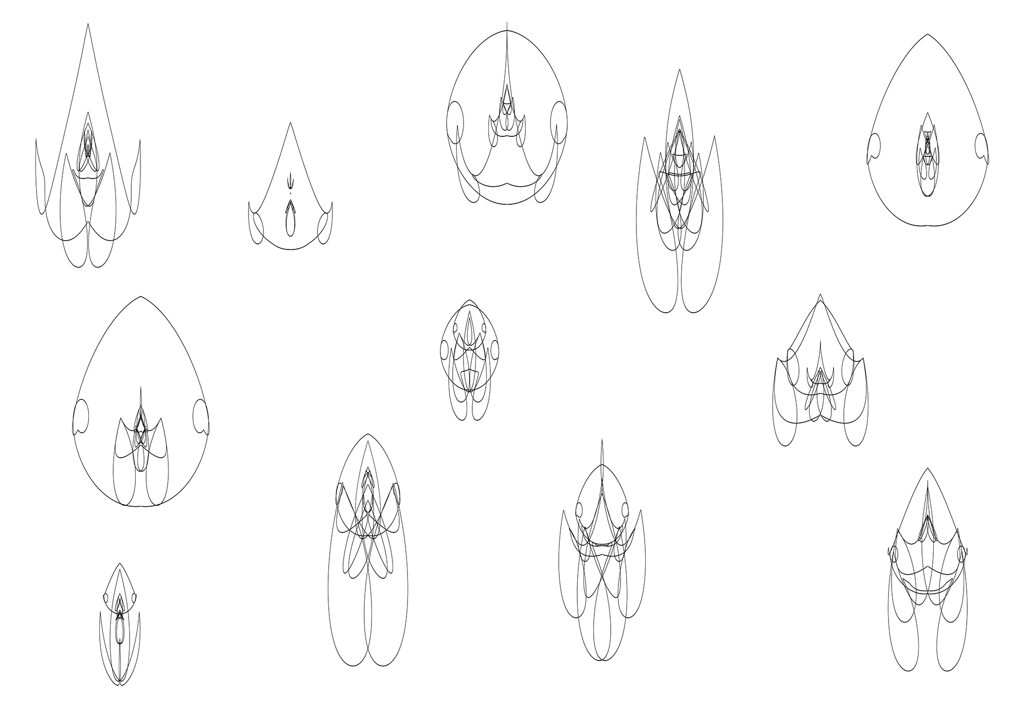
Note each of the above plots is actually the result of $4$ randonly generated plots on top of one another and increasingly offset on the $y$ axis (slightly).
Interactive Version
Click the below plot - values $a$ through $e$ will be randomized.
Again, this is $4$ plots on top of one another. To render this plot with a single layer hold your shift key and click.
The Scarabaeus and Cornoid
The original equation for the Scarabaeus curve in polar coordinates is:
... and the Cornoid in parametric form:
Quick Background
The original impetus for the creation of the Insectoid Curve was to create a curve that had features similar to an insect - specifically a beatle. After combining the Cornoid and Scarabaeus the result you see here came about rather quickly.